Logistic Regression with L1 Regularization
Let Y denote the response variable. $Y$ is a 0-1 valued variable with a success coded as a 1. Let $X = (X_1 . . . X_m)$ denote the values of the $m$ predictors.
The odds ratio $O$ is defi ned as:
$$O = {Pr(Y = 1|X) \over 1- Pr(Y = 1|X)}$$
The logistic regression model assumes that the log-odds ratio is related to the predictors by:
$$\mathrm{logit} = \log(O) = \beta_0 + \beta_ 1X_1 + ... + \beta_ mX_m$$
The slope parameters in this model have a meaningful interpretation.
Consider $\beta_1$: If we increase $X_1$ by one unit while holding the other predictors fi xed, exp( $\beta_1$) is the resulting change in the odds for success. If $\beta_1 = 0.693$, the odds of success doubles when $X_1$ increases by one unit $\exp(0.693) = 2$.
The logistic regression model can also be used to classify observations. We classify an observation as a success, $Y=1$, if $\Pr(Y=1|X) \ge 0.5$. This is the same as classifying an observation as a success if the $\mathrm{logit} \ge 0$. Changing the value of the threshold 0 can lead to classifiers with different behavior.
Classification Matrix

The precision is the fraction of positive predictions made that were correct. The recall, or sensitivity, is the true positive rate for each class. It is the fraction of positive results that were classified as positive.
The Fitting Criterion
Given a data set $(Y_1,X_1), . . . , (Y_n,X_n)$, the usual method of fitting the logistic regression model minimizes a criterion of the form: $$\mathrm{Dev}( \beta) = -2n^{-1} \log \prod_{Y_i=1} \Pr(Y_i | X_i;\beta ) \prod_{Y_i=0} \Pr(Y_i | X_i; \beta )$$ When the dimension of $X$ is large, the fit can become unstable resulting in predictions with large variance. We can regularize the fit by adding a term to the fitting criterion which penalizes large values of $\beta$. One penalty term that is often incorporated is the so-called LASSO penalty. The penalized criterion is $$\mathrm{Dev}( \beta) + \lambda \sum_{j=1}^m|\beta_j|$$ When $\lambda = 0$, there is no penalty. As $\lambda$ grows, the estimated coefficients are shrunk towards 0. Scikit-Learn's logistic regression classifier, uses a penalty term that is the reciprocal of $\lambda$.
L1-regularization path
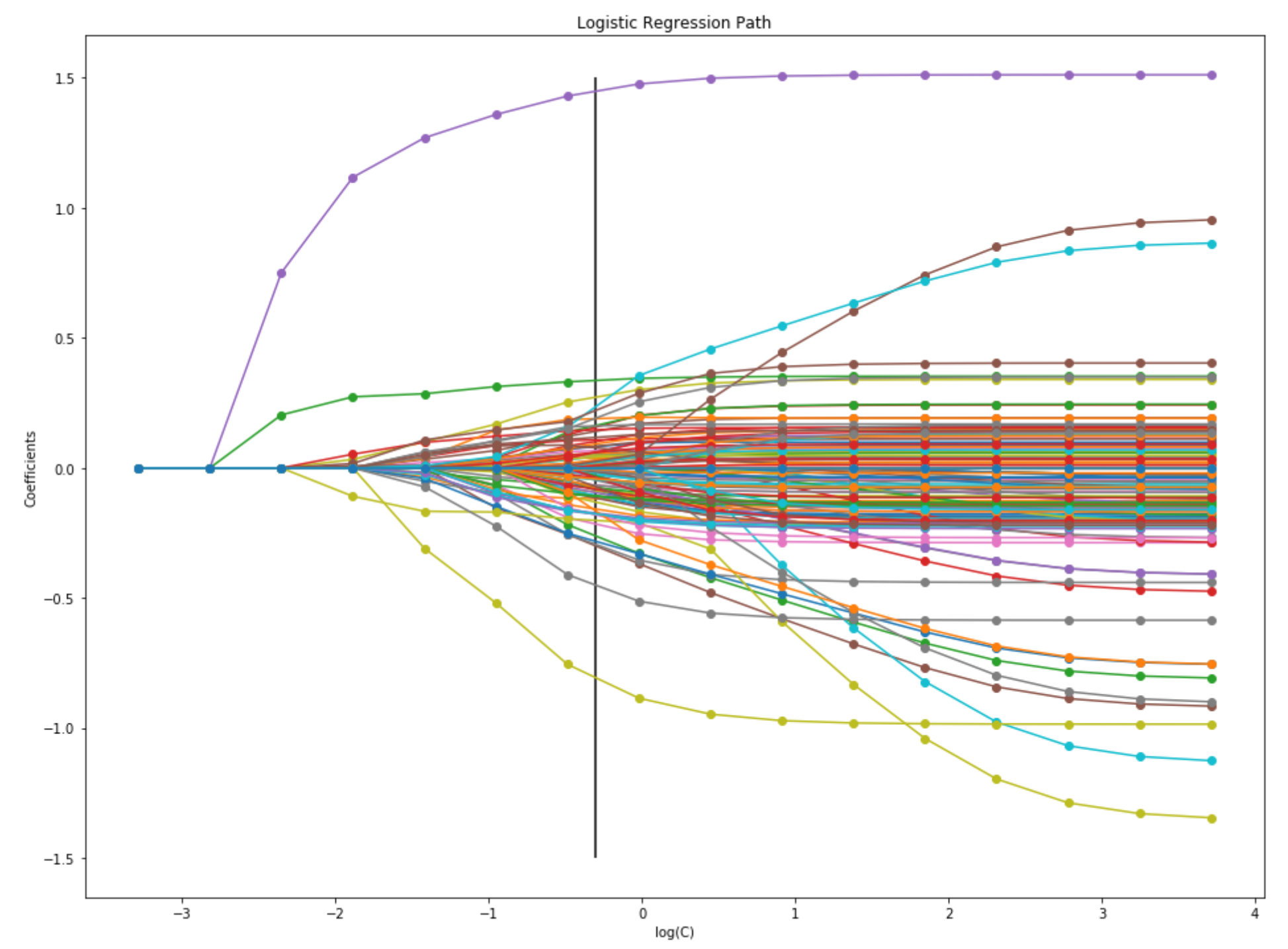
Moving from right to left, the paths show how the parameters shrink with the increasing penalization.
The vertical line at C = 0.5 corresponds to the best parameter choice as found by GridSearchCV.
Credit: Alexandre Gramfort
ROC Curve of Classifier
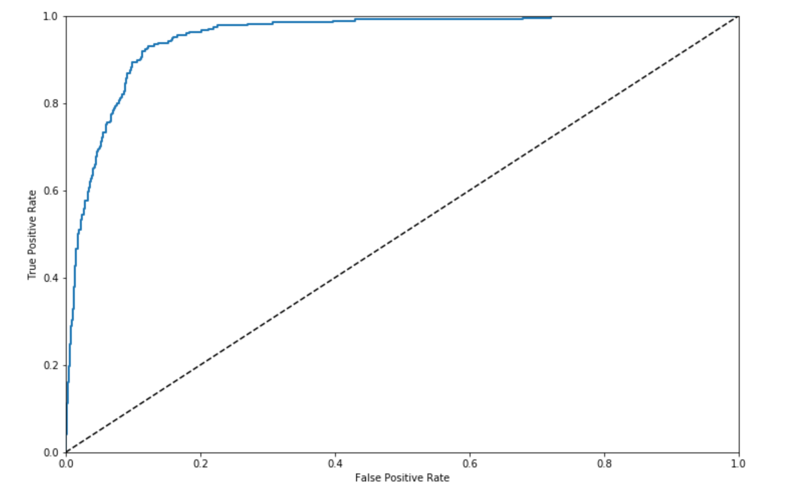
The receiver operating characteristic curve displays the trade-off between the True Positive Rate (recall) and the False Positive Rate. A classifier that guesses at random would fall somewhere on the dotted line. A perfect classifier would be at the point (0, 1) in the upper left-hand corner: No False Negatives and No False Positives.
Precision and Recall as a Function of the Threshold
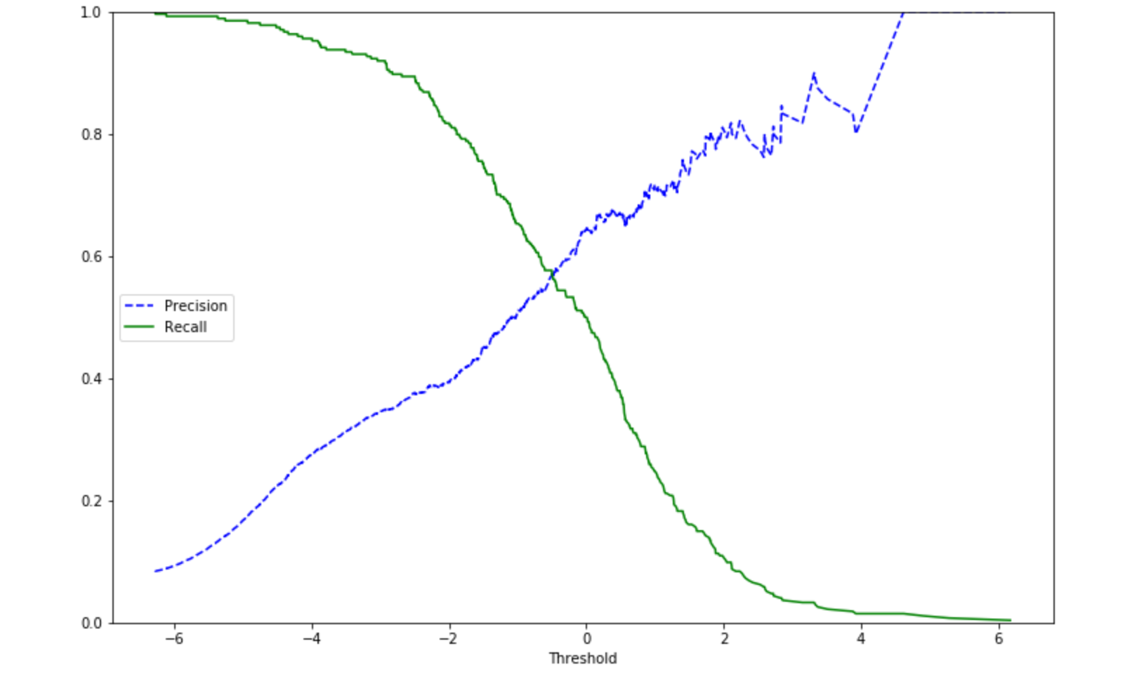
By adjusting the threshold that our classifier uses, we can adjust the recall of our classifier. This will be at the expense of the precision; however, in this problem, correctly classifying an individual that would attempt suicide (True Positive) is more important than having more false positives. For example, if we use a threshold of -2, our classifier would have a recall 0.82 and a precision of 0.39 within the the Attempt = Yes class.